Matrices and Portfolio Variance

Matrices are widely used in portfolio theory, financial economics, and econometrics because of the need to manipulate significant data inputs. 

In this article, you will learn core matrix operations and how portfolio variance, widely used in portfolio allocation decisions, can be represented in the matrix form and implementations in R, Julia, and Python languages. 

1. Matrix operations

2. Portfolio variance in matrix form

3. Implementation in R, Julia, and Python

1. Matrix Operations

Matrices are valuable and essential ways of organizing data sets, which makes manipulating and transforming them much more straightforward.

Terminology

• Scalar: a single number. E.g., 3, 5.5

• Vector: one-dimensional array of numbers

• Matrix: a 2D collection of arrays

A vector is a special matrix case with only one column or row.

• If a matrix has only one row, it’s known as a row vector with a dimension of 1 x C

• If a matrix has only one column, it’s known as a column vector with a dimension of R x 1

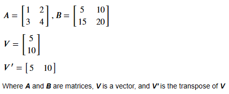
Matrix Definition

Let’s start by defining two matrices and one vector we will use throughout this section.

### R
A = matrix(c(1, 2, 3, 4), nrow = 2, ncol = 2, byrow = TRUE)
B = matrix(c(5, 10, 15, 20), nrow = 2, ncol = 2, byrow = TRUE)
V = c(5, 10)

### Julia
A = [1 2;  3 4] # 2x2 matrix
B = [5 10; 15 20] # 2x2 matrix
V = [5, 10] # vector

### Python
import numpy as np
A = np.array([[1, 2], [3,4]]) # 2x2 matrix
B = np.array([[5, 10], [15,20]]) # 2x2 matrix
V = np.array([5, 10]) # vector

Addition

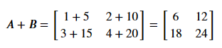
# You can add matrices with the same size

### R, Julia, Python
A + B

Subtraction

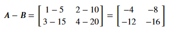
# You can subtract matrices with the same size

### R, Julia, Python
A - B

Multiplication

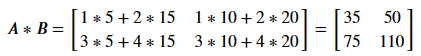
### R
A %*% B # Not A * B

### Julia
A * B

### Python
np.dot(A, B)

Matrix-Scalar Multiplication

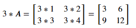
### R, Julia, Python
3 * A
# + 3A in Julia

Matrix-Vector (Transposed) Multiplication

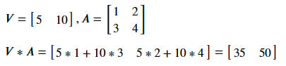
### R
t(V) %*% A

### Julia
V' * A

### Python
np.dot(V.T, A) 

Matrix-Vector Multiplication

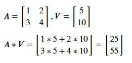
### R
A %*% V

### Julia
A * V

### Python
np.dot(A, V)

2. Portfolio Variance in Matrix Form

Modern portfolio theory (MPT) states that portfolio variance can be reduced by selecting securities with low or negative correlations in which to invest, such as stocks and bonds. (Investopedia)

Modern Portfolio Theory is not the main subject of this article, therefore skipping its details here. In another post, I will explain modern portfolio theory in detail with R, Julia, and Python implementation.

Matrix form of two-asset portfolio variance

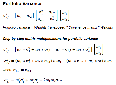
The illustration in the image above is for the two-asset portfolio, but using the same matrix form, you can extend it to any number of assets.

In more plain language, what we need to calculate is:

Portfolio variance = Weights transposed * Covariance matrix *Weights

3. Implementation in R, Julia, and Python

R Implementation

weights = c(0.6, 0.4)

covMatrix = matrix(
  c(0.000738889, 0.000538889, 0.000538889, 0.00549889),
  nrow = 2,
  ncol = 2,
  byrow = TRUE
)

portVar = t(weights) %*% covMatrix %*% weights
portStd = sqrt(portVar)

print(paste("Portfolio Variance is: ", portVar))
print(paste("Portfolio Risk (Std) is: ", portStd))

Julia Implementation

weights = [0.6, 0.4]

covMatrix = [0.000738889 0.000538889; 0.000538889 0.00549889]
portVar = weights' * covMatrix * weights
portStd = sqrt(portVar)

print("Portfolio Variance is $portVar")
print("Portfolio Risk (Std) is $portStd")

Python Implementation

import numpy as np
weights = np.array([0.6, 0.4])
covMatrix = [[0.000738889, 0.000538889],
             [0.000538889, 0.00549889]]

portVar = np.dot(np.dot(weights, covMatrix), weights.T)
portStd = np.sqrt(portVar)
print("Portfolio Variance: ", portVar)
print("Portfolio Risk (Std): ", portStd)